Example 5A: Parameter sweep
Info
Metropolis searches are applied to find an appropriate temperature range for parallel tempering. Don't know what Metropolis search is? Read this. Never heard about parallel tempering? Read this.This example demonstrates how to find an appropriate temperature range for parallel tempering using the automated analysis workflow from the extensions module. The core subset selection problem from example 1C is used as a case study. Several Metropolis searches with different fixed temperatures are applied. The results are then inspected using the provided R package, to infer an appropriate temperature range to be used for the parallel tempering algorithm.
Analysis setup
To find an appropriate temperature range for the parallel tempering algorithm, we will run several Metropolis searches with different temperatures and assess their performance for a series of datasets. Each dataset consists of a distance matrix based on which the entry-to-nearest-entry score of any considered subset is computed (see example 1C). This score is to be maximized. To execute the algorithms and gather statistics about the obtained solution quality, convergence, etc. we will use the analysis workflow included in the extensions module. This requires to add this module as a dependency to your project, in addition to the core module.
The first step is to create an analysis object, specifying the solution type of the problems that will be analyzed.
// initialize analysis object
Analysis<SubsetSolution> analysis = new Analysis<>();
Then, the problems are added. In this example there is one problem for each
considered dataset and they all have the same entry-to-nearest-entry objective. Data is read
from CSV files using the CoreSubsetFileReader which is included in the full
source code
of example 1A where the corresponding data type
CoreSubsetData is also defined. The implementation of the
EntryToNearestEntryObjective is described in example 1C.
The size of the constructed core is determined relative to the size of the full dataset by specifying a fixed selection ratio (e.g. 0.2). Every analyzed problem needs to be assigned a unique ID (string). Here, the file name is used as the ID (without directories and without extension).
// set input file paths
List<String> filePaths = Arrays.asList("my/input/file1.csv", "my/input/file2.csv", ...);
// read datasets
CoreSubsetFileReader reader = new CoreSubsetFileReader();
List<CoreSubsetData> datasets = new ArrayList<>();
for(String filePath : filePaths){
  datasets.add(reader.read(filePath));
}

// create objective
EntryToNearestEntryObjective obj = new EntryToNearestEntryObjective();

// set selection ratio
double selRatio = 0.2;
// add problems (one per dataset)
for(int d = 0; d < datasets.size(); d++){
    // create problem
    CoreSubsetData data = datasets.get(d);
    int coreSize = (int) Math.round(selRatio * data.getIDs().size());
    SubsetProblem<CoreSubsetData> problem = new SubsetProblem<>(data, obj, coreSize);
    // set problem ID to file name (without directories and without extension)
    String path = filePaths.get(d);
    String filename = new File(path).getName();
    String id = filename.substring(0, filename.lastIndexOf("."));
    // add problem to analysis
    analysis.addProblem(id, problem);
}
Ten Metropolis searches are then added to the analysis, each with a unique ID and different fixed temperature,
equally spread across a given interval [minTemp, maxTemp]. Note that the method
addSearch(id, searchFactory) requires to specify a search factory.
This is because each algorithm will be executed several times and for each such run a new search
instance is created, using the given factory. The search factory interface is a functional interface
with a single method create(problem) to create a search that solves the given problem.
A search factory can therefore easily be specified with a Java 8 lambda expression, as in the example
code below. The same stop criterion is used here for every generated search (maximum runtime of 5 minutes).
// create stop criterion
long timeLimit = 300;
StopCriterion stopCrit = new MaxRuntime(timeLimit, TimeUnit.SECONDS);

// set temperature range
double minTemp = ...
double maxTemp = ...
// set number of Metropolis searches
int numSearches = 10;
// create and add searches
double tempDelta = (maxTemp - minTemp)/(numSearches - 1);
for(int s = 0; s < numSearches; s++){
    // set temperature
    double temp = minTemp + s * tempDelta;
    // add Metropolis search
    String id = "MS-" + (s+1);
    analysis.addSearch(id, problem -> {
        Search<SubsetSolution> ms = new MetropolisSearch<>(problem, new SingleSwapNeighbourhood(), temp);
        ms.addStopCriterion(stopCrit);
        return ms;
    });
}
By default, every search is executed 10 times (in addition to a single burn-in run).
The number of runs can be changed using the method setNumRuns(n).
// run searches 5 times
analysis.setNumRuns(5);
If desired, the number of burn-in runs can also be customized with setNumBurnIn(n).
Results of these preliminary runs are discarded. Both settings can also be adjusted at a
search specific level using setNumRuns(searchID, n) and
setNumBurnIn(searchID, n).
Run analysis
Now that the analysis has been set up, we are ready to run it.
AnalysisResults<SubsetSolution> results = analysis.run();
Be patient
Wait a while for the analysis to complete. In the example setup from above, each of the 10 Metropolis searches is executed 6 times (5 registered runs + 1 additional burn-in). Every run takes 5 minutes and the entire analysis is repeated for each dataset. This yields an expected runtime of about 5 hours per dataset.Track progress
While an analysis is running, log messages are produced to report the progress. All messages are tagged with a marker"analysis" so that they can be filtered from other messages when using a marker aware logging
framework (such as logback). To pick up log messages, follow
these instructions.
The results of the analysis are packed into an object of type AnalysisResults.
For every combination of an applied search and analyzed problem, the progress of each performed
search run and corresponding final best found solution are reported. The results of
a specific run can be retrieved with
SearchRunResults<SubsetSolution> run = results.getRun("problemID", "searchID", i);
using the IDs that have been assigned to the problem and search during setup, where i
indicates the search run index (a value in [0, n-1] when n search runs have
been performed). From the returned object, the times at which a new best solution
was found and the corresponding evaluation values can be retrieved, as well as the final best solution
obtained in this search run.
Although the results can be directly accessed as described above, the easiest way to inspect them is through the provided R package. To do this, first write the results to a JSON file.
results.writeJSON("sweep.json", JsonConverter.SUBSET_SOLUTION);
The second argument specifies how to convert solutions to JSON format. For subset selection problems,
the predefined JsonConverter.SUBSET_SOLUTION can be used, defined as
sol -> Json.array(sol.getSelectedIDs().toArray())
Given a subset solution, the predefined converter creates a JSON array containing the IDs of the selected items. To write your own JSON converters, take a look at the mjson library. If no converter is given, the output file will not contain the actual best found solutions but only report the progress in terms of obtained evaluation value over time.
Inspect results
The obtained JSON file can be loaded into R using the provided R package. The package can be installed from CRAN with
> install.packages("james.analysis")
and loaded with
> library(james.analysis)
Running the analysis with a minimum and maximum temperature of 10‑8 and 10‑3, respectively, on
4 datasets
(one coconut, two maize and one pea collection)
produced the file
sweep-0.001.json.
It can be loaded into R with the function readJAMES.
> sweep <- readJAMES("sweep-0.001.json")
Printing a summary with
> summary(sweep)
reveals the 4 analyzed datasets and the 10 applied Metropolis searches. For each combination of an analyzed problem and applied search, the summary reports the number of executed search runs and the mean and median value obtained in those runs, together with the corresponding standard deviation and interquartile range.
Problem:         Search:  Runs:  Mean value:  St. dev:   Median:      IQR:
---------------  -------  -----  -----------  --------  --------  --------
coconut          MS-1         5         0.57  0.000474      0.57  0.000521
coconut          MS-2         5        0.564   0.00019     0.564   0.00034
coconut          MS-3         5        0.545  0.000813     0.545  0.000706
coconut          MS-4         5         0.53  0.000772      0.53  0.000979
coconut          MS-5         5        0.522  0.000752     0.522   0.00117
coconut          MS-6         5        0.515  0.000861     0.515   0.00109
coconut          MS-7         5        0.512  0.000811     0.512  0.000549
coconut          MS-8         5        0.509  0.000498     0.509  0.000855
coconut          MS-9         5        0.506  0.000657     0.505  0.000862
coconut          MS-10        5        0.504   0.00131     0.505   0.00148
maize-accession  MS-1         5        0.576  0.000397     0.576  0.000271
maize-accession  MS-2         5        0.578    0.0001     0.578  8.32e-05
maize-accession  MS-3         5        0.571  0.000268     0.571  0.000137
maize-accession  MS-4         5        0.564    0.0012     0.564   0.00139
maize-accession  MS-5         5        0.556   0.00113     0.556   0.00059
maize-accession  MS-6         5         0.55  0.000902      0.55   0.00131
maize-accession  MS-7         5        0.545  0.000872     0.545  0.000276
maize-accession  MS-8         5        0.542  0.000581     0.542  0.000705
maize-accession  MS-9         5        0.537  0.000535     0.537  0.000958
maize-accession  MS-10        5        0.535   0.00135     0.534   0.00226
maize-bulk       MS-1         5         0.43  0.000101      0.43  4.02e-05
maize-bulk       MS-2         5         0.43  8.94e-16      0.43  9.99e-16
maize-bulk       MS-3         5         0.43  8.36e-16      0.43  9.99e-16
maize-bulk       MS-4         5         0.43  0.000104      0.43  7.05e-15
maize-bulk       MS-5         5        0.429  0.000276     0.429  0.000265
maize-bulk       MS-6         5        0.428  0.000721     0.428  0.000548
maize-bulk       MS-7         5        0.426  0.000617     0.426  0.000857
maize-bulk       MS-8         5        0.422  0.000492     0.422  0.000383
maize-bulk       MS-9         5        0.418  0.000931     0.418   0.00143
maize-bulk       MS-10        5        0.415   0.00188     0.414   0.00204
pea-small        MS-1         5        0.353  0.000761     0.353   0.00135
pea-small        MS-2         5        0.346  0.000301     0.346  0.000285
pea-small        MS-3         5        0.322   0.00106     0.322   0.00123
pea-small        MS-4         5        0.303   0.00112     0.302  0.000566
pea-small        MS-5         5        0.291   0.00107     0.291   0.00189
pea-small        MS-6         5        0.281    0.0016     0.281  0.000265
pea-small        MS-7         5        0.274   0.00062     0.274  0.000846
pea-small        MS-8         5        0.268   0.00113     0.268   0.00129
pea-small        MS-9         5        0.263  0.000811     0.263  0.000542
pea-small        MS-10        5         0.26   0.00182      0.26   0.00128
To get a better overview of how the temperature influences the solution quality, we can draw box plots with the function boxplot.
> temp.range <- seq(1e-8, 1e-3, length.out = 10)
> x <- "Temperature"
> boxplot(sweep, problem = "coconut", names = temp.range, xlab = x)
> boxplot(sweep, problem = "maize-accession", names = temp.range, xlab = x)
> boxplot(sweep, problem = "maize-bulk", names = temp.range, xlab = x)
> boxplot(sweep, problem = "pea-small", names = temp.range, xlab = x)
This produces the following visualizations:
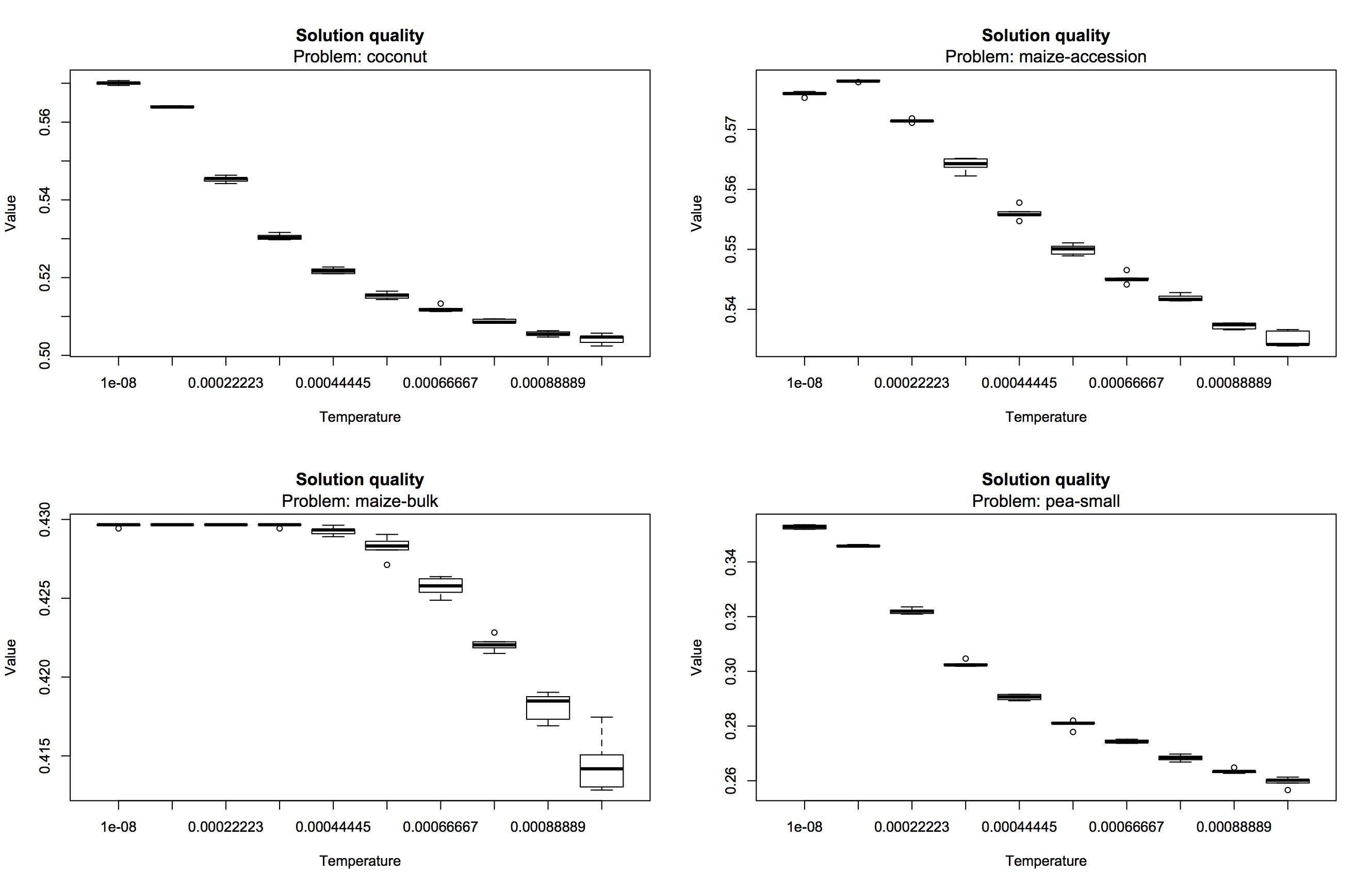
For three of the analyzed datasets, the solution quality consistently drops when increasing the temperature. Only for one of both maize collections (maize-accession) there is a slight increase in performance at a temperature of about 10‑4, followed by a large decrease. These results suggest that we might have set the maximum temperature too high. So let's try again with a lower maximum temperature of 10‑4 (and the same minimum of 10‑8). This produces the output file sweep-0.0001.json.
> sweep2 <- readJAMES("sweep-0.0001.json")
> temp.range <- seq(1e-8, 1e-4, length.out = 10)
> x <- "Temperature"
> boxplot(sweep2, problem = "coconut", names = temp.range, xlab = x)
> boxplot(sweep2, problem = "maize-accession", names = temp.range, xlab = x)
> boxplot(sweep2, problem = "maize-bulk", names = temp.range, xlab = x)
> boxplot(sweep2, problem = "pea-small", names = temp.range, xlab = x)
The box plots now look like this:
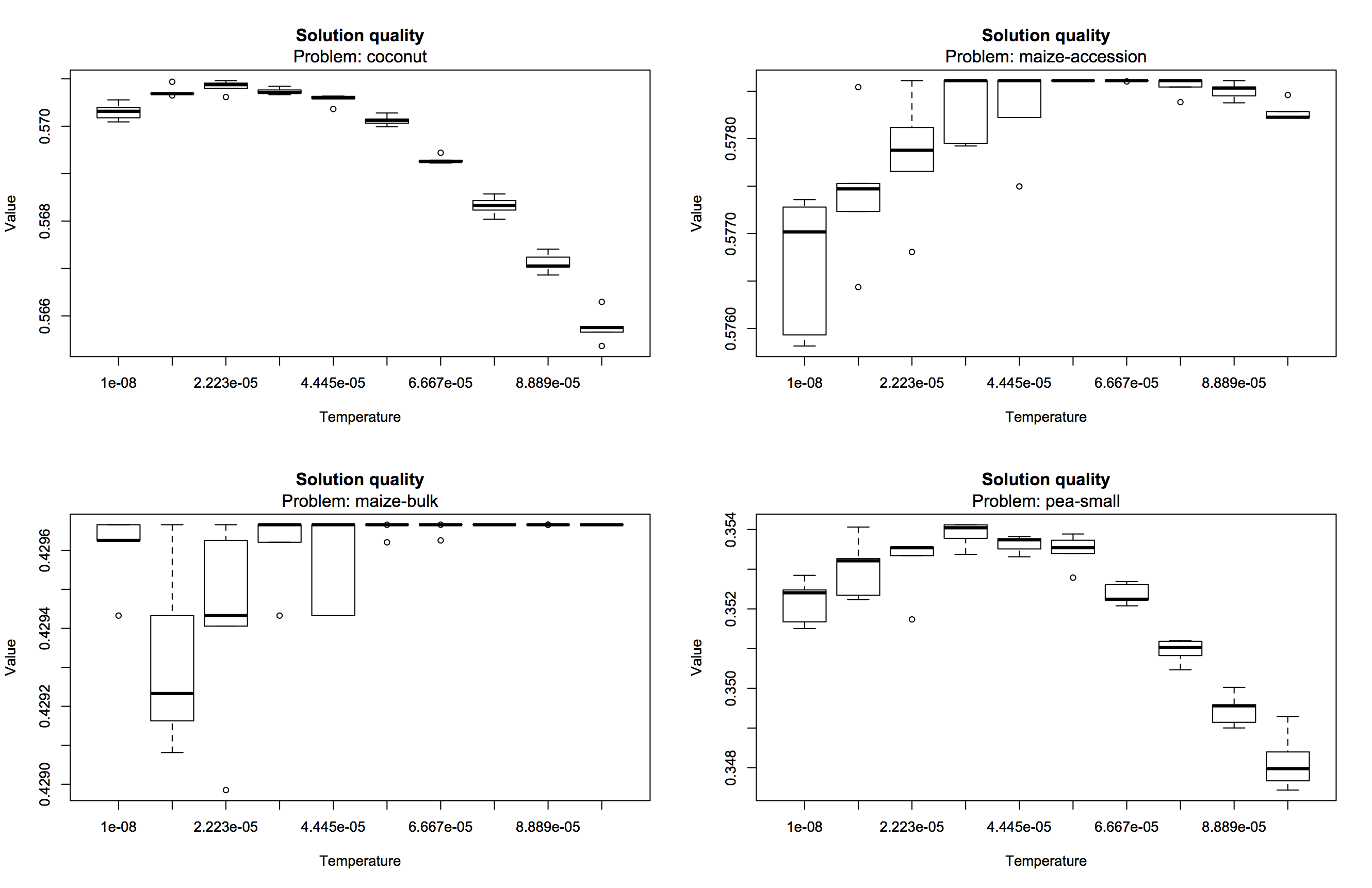
When increasing the temperature there is now clearly an initial rise in solution quality, and a reduction of variability across runs, for each analyzed dataset. For all datasets except one maize collection (maize-bulk) this rise is followed by a moderate performance drop, which is not necessarily undesired. In a parallel tempering approach, these warmer replicas increase the power to escape from local optima. Yet the search strategy cannot solely be based on lucky shots so that this range of [10‑8, 10‑4] is a better choice than the first attempt with a higher maximum temperature of 10‑3.
Example 5B actually applies parallel tempering with the chosen temperature range of [10‑8, 10‑4] and compares its performance with that of a basic random descent algorithm.
Full source code
The complete source code of this example is available on GitHub. You can also download a ZIP file that contains the Java sources of all examples, a compiled JAR (including all dependencies) as well as some input files for in case you want to run any of the examples. To run this example, execute
$ java -cp james-examples.jar org.jamesframework.examples.analysis.ParameterSweep <selectionratio> <runs> <runtime> <mintemp> <maxtemp> <numsearches> [ <inputfile> ]+from the command line. The selection ratio determines the core size. The following arguments specify the number of runs (repeats) that will be performed for each search, the runtime limit (in seconds) of each run, the minimum and maximum temperature and the actual number of Metropolis searches (i.e. number of considered temperatures). The input files (at least one) should be CSV files in which the first row contains N item names and the subsequent N rows specify an N × N distance matrix. The analysis will be repeated for each dataset loaded from the given files. All output is combined into a single file
sweep.json that
can be loaded in R using the provided R package.