Javadoc API

A fully specified Javadoc API is provided for the core and extensions module.

Latest stable API

Consult the latest stable APIs:

• Core module API (1.2)
• Extensions module API (1.2)

Previous versions are found here.

Development snapshots

Bleeding edge development snapshot APIs are also available:

• Core module API (1.3-SNAPSHOT)
• Extensions module API (1.2.1-SNAPSHOT)

Problem specification

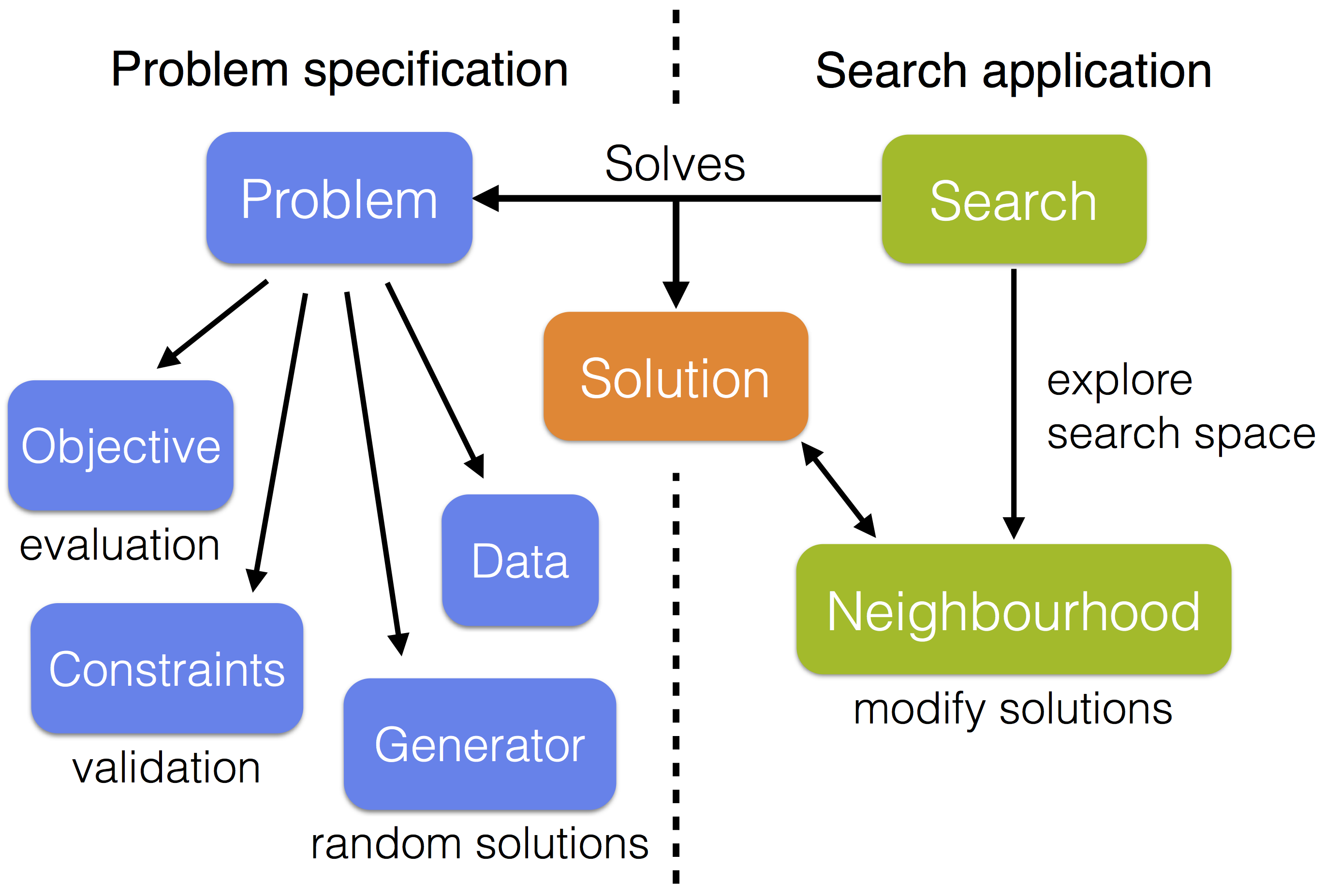
The JAMES framework strongly separates problem specification from search application so that existing algorithms can easily be applied to obtain solutions for newly implemented problems. Each problem has a specific solution type and a search creates solutions of this type to solve the problem. The search communicates with the problem to obtain random solutions (e.g. used as the default initial solution of a local search) and to evaluate and validate constructed solutions.

Some utilities are provided to split the problem specification into data, an objective, any number of constraints and a random solution generator. The objective and constraints are then responsible for evaluating and validating solutions, using the data, respectively. Most available optimization algorithms are local searches that repeatedly modify the current solution in an attempt to improve it. To use these searches it is necessary to provide at least one neighbourhood, which generates moves that are applied to the current solution. The neighbourhood(s) should be compatible with the solution type of the problem that is being solved.

The core module contains predefined components for subset selection problems, including a predefined solution type, a high-level problem specification with a built-in random subset generator, and several subset neighbourhoods. Similar components can easily be created for other types of problems. Some are provided in the extensions module.

Subset selection

The provided subset selection components require that a unique integer ID is assigned to each item in the data set. Any subset selection problem is then translated into selection of a subset of IDs. Follow these steps to implement a subset selection problem:

1. Create a custom data class (e.g. MyData) by implementing the IntegerIdentifiedData interface. This interface defines a single method getIDs() that returns the set of all IDs assigned to an item in the data set. Also add the necessary custom methods to access (properties of) items based on their IDs.
2. Provide an objective function by implementing the Objective interface. This is a generic interface with two type parameters: the solution and data type. Set the solution type to SubsetSolution and the data type to MyData. Now implement the necessary methods to evaluate solutions using the underlying data and to inform the search whether evaluations are to be minimized or maximized. If desired, an efficient delta evaluation can also be provided, to evaluate a neighbour of the current solution of a local search based on its current evaluation and the applied move.
3. Specify the constraints (if any) by implementing the Constraint and/or PenalizingConstraint interfaces, to be added as mandatory and/or penalizing constraints to the problem definition. Solutions that do not satisfy all mandatory constraints are discarded. If a penalizing constraint is violated, a penalty is assigned to the solution's evaluation but the solution is still considered as valid. Both interfaces again have a generic solution and data type which should be set to SubsetSolution and MyData, respectively. Efficient delta validations can also be provided (optional).
4. Combine the data, objective and constraints (if any) in a SubsetProblem. The desired minimum and maximum (or fixed) subset size can be specified. The data and objective are required and set at construction while mandatory and penalizing constraints can be added later using addMandatoryConstraint(c) and addPenalizingConstraint(c), respectively.

The problem definition can be passed to any local search to optimize the selection. Several predefined subset neighbourhoods are available which add and/or remove some IDs to/from the selection to modify the current solution. Note that some searches may require additional parameters or components to be specified. Details are best explained through some examples.

Beyond subset selection

Other types of problems can also be easily modeled and solved:

1. Define a custom solution type, say MySolution, by extending the abstract Solution class.
2. Create a custom data class, say MyData, containing the data required for evaluation, validation and/or random solution generation. The data type is not restricted in any way, i.e. it is not required to implement a specific interface or extend an (abstract) class. So it is entirely up to you to decide how the data is represented.
3. Implement the objective and constraints (if any) by following the same steps as for a subset selection problem (see above), but now with solution and data type MySolution and MyData, respectively.
4. Provide a random solution generator, implementing the RandomSolutionGenerator interface, again with solution and data type MySolution and MyData, respectively. The generated random solutions are for example used to obtain a default initial solution when applying a local search.
5. Combine the data, objective, constraints (if any) and random solution generator in a GenericProblem with solution and data type MySolution and MyData, respectively.
6. Provide at least one implementation of the Neighbourhood interface with solution type MySolution. A neighbourhood generates moves that can be applied to a solution to modify it and undone to go back to the previous solution. All moves implement the Move interface.

The composed problem can now be solved with any of the available local searches, using the defined neighbourhood(s) to modify the solution. Note that some searches may require additional parameters or components to be specified. Examples are provided here.

Optimization algorithms

All available algorithms that can be used to obtain solutions for the specified problems are listed here. Most algorithms are local search metaheuristics, with a few exceptions such as exhaustive search and one heuristic specifically designed for subset sampling. Some basic building blocks for hybrid (parallel) searches are also provided.

If you do not know what a local search metaheuristic is, read this.

Most local search algorithms use one ore more neighbourhood(s) to explore the search space, starting from a random (or manually specified) initial solution. A neighbourhood defines a set of solutions similar to the current solution that can be obtained by applying small changes (moves) to this current solution. Such moves are repeatedly applied to the current solution in an attempt to improve it. Therefore, the chosen neighbourhoods strongly influence the behaviour of the search algorithms.

Random descent

Random descent is the most basic local search algorithm (also called stochastic hill climbing). In every step, a random neighbour of the current solution is evaluated and accepted as the new current solution if and only if it is valid and better than the current solution.

Random descent does not terminate internally. Therefore, a stop criterion should be specified, such as a maximum number of steps or a maximum runtime. By default, the search starts with a random initial solution. Alternatively, a custom initial solution can be specified. Any neighbourhood that is compatible with the solution type of the considered problem can be applied.

Random descent (API version: 1.2)

Steepest descent

Steepest descent (also referred to as hill climbing) is a local search algorithm that always accepts the best valid neighbour of the current solution as the new current solution, until no more improvement is made.

By default, the search starts with a random initial solution. Alternatively, a custom initial solution can be specified. Any neighbourhood that is compatible with the solution type of the considered problem can be applied.

Steepest descent (API version: 1.2)

Tabu search

Tabu Search is based on steepest descent but does not require that an improvement is made in every step. The best valid non-tabu neighbour of the current solution is always accepted as the new current solution. This may allow the search to escape from a local optimum.

To avoid repeatedly revisiting the same solutions (i.e. traversing cycles in the solution space) the neighbourhood is dynamically modified using a tabu memory. This memory keeps track of recently visited solutions, presence of specific features in these solutions and/or recently modified features (recently applied moves). Based on this memory, specific solutions are declared tabu and are removed from the neighbourhood to favour unvisited regions which may contain new improvements.

The search terminates internally if all valid neighbours of the current solution are tabu. However, as this may never happen, a stop criterion should preferably be specified to guarantee termination. By default, the search starts with a random initial solution. Alternatively, a custom initial solution can be specified. Any neighbourhood that is compatible with the solution type of the considered problem can be applied.

Tabu search (API version: 1.2)

Metropolis search

Metropolis search is an extension of random descent where a valid neighbour that is no improvement over the current solution may still be accepted as the new current solution. The probability to accept such inferior neighbour is proportional to both

1. the difference of its evaluation compared to that of the current solution, and
2. the temperature of the search.

A higher temperature yields a higher probability to accept inferior moves. Thus, a high temperature allows a lot of freedom to escape from local optima, while lower temperatures ease convergence towards an optimum.

The basic Metropolis search implementation in JAMES has a fixed temperature. It may therefore not be very useful on its own, but it is for example used by the more advanced parallel tempering algorithm. Also, it can provide useful insights in the performance of different temperatures for a specific application.

Metropolis search does not terminate internally. Therefore, a stop criterion should be specified, such as a maximum number of steps or a maximum runtime. By default, the search starts with a random initial solution. Alternatively, a custom initial solution can be specified. Any neighbourhood that is compatible with the solution type of the considered problem can be applied.

Metropolis search (API version: 1.2)

Parallel tempering

Parallel tempering (also referred to as Replica Exchange Monte Carlo) is an advanced local search algorithm that concurrently runs several Metropolis searches with different temperatures. Each of these subsearches repeatedly apply a series of moves on a private solution and the global best solution found by any replica is tracked by the main search. The parallel tempering algorithm is somewhat similar to simulated annealing but takes advantage of modern multi-core architectures and is generally less sensitive to parameter values such as replica temperatures, as compared to e.g. the initial temperature and cooling scheme in simulated annealing.

When applying the parallel tempering algorithm, the number of replicas and a minimum and maximum temperature have to be set. Temperatures assigned to replicas are equally spaced in the specified interval and replicas are ordered according to their temperature. Between consecutive runs of the Metropolis searches, solutions of neighbouring replicas are swapped to push the most promising solutions towards the lowest temperatures, for the sake of convergence, while inferior solutions are shifted to hot replicas where they can be extensively modified in an attempt to find further improvements. In this way, the hot replicas continuously provide new seeds for the cooler replicas.

The parallel tempering algorithm does not terminate internally. Therefore, a stop criterion should be specified, such as a maximum number of steps or a maximum runtime. Keep in mind that every step of parallel tempering consists of a number of steps performed by each Metropolis search. By default, every replica starts with an independently generated random initial solution. Alternatively, a custom initial solution can be specified (global, or per replica through a custom Metropolis search factory). Any neighbourhood that is compatible with the solution type of the considered problem can be applied.

Note that all Metropolis searches are executed in separate threads to take advantage of multi-core architectures.

Parallel tempering (API version: 1.2)

Variable neighbourhood descent

Variable neighbourhood descent (VND) is an extension of steepest descent which uses a series of neighbourhoods N₁, ..., N_k. The search starts as a steepest descent using neighbourhood N₁. When this neighbourhood does not contain any improvement (local optimum) the other neighbourhoods N₂, ..., N_k are explored one by one. If an improvement is found in one of these alternative neighbourhoods, the algorithm switches back to neighbourhood N₁ and continues from the new current solution, else, the search terminates.

Combining several neighbourhoods can be beneficial because a local optimum for one neighbourhood is not necessarily a local optimum for an other neighbourhood. Often, neighbourhoods of increasing size are chosen so that the smallest neighbourhood is most frequently applied, for efficiency, while the larger neighbourhoods still offer a way out of local optima of the smaller neighbourhoods.

By default, the search starts with a random initial solution. Alternatively, a custom initial solution can be specified. Any series of neighbourhoods that are compatible with the solution type of the considered problem can be applied.

Variable neighbourhood descent (API version: 1.2)

Reduced variable neighbourhood search

Reduced variable neighbourhood search (RVNS) is a random descent based algorithm that uses a series of neighbourhoods N₁, ..., N_k. It iteratively samples a random neighbour from the current neighbourhood N_i (initially starting with N₁). If this neighbour is no valid improvement over the current solution, a new neighbour is sampled using the next neighbourhood N_i+1 in the subsequent step. Else, the neighbour is accepted as the new current solution and the neighbourhood is reset to N₁.

By default, when a neighbour obtained from the last neighbourhood N_k is not accepted, RVNS cyclically continues with neighbourhood N₁ as some neighbourhoods may not yet have been fully explored due to random sampling. If desired, this neighbourhood cycling can be disabled in which case the search terminates when one neighbour of the current solution has been sampled from every neighbourhood, without finding an improvement.

Except when neighbourhood cycling is disabled, reduced variable neighbourhood search never terminates internally. Therefore, a stop criterion should be specified, such as a maximum number of steps or a maximum runtime. By default, the search starts with a random initial solution. Alternatively, a custom initial solution can be specified. Any series of neighbourhoods that are compatible with the solution type of the considered problem can be applied.

Reduced variable neighbourhood search (API version: 1.2)

Variable neighbourhood search

Variable neighbourhood search (VNS) is a more advanced multi-neighbourhood search compared to VND and RVNS. It applies a combination of a series of neighbourhoods for random shaking and an arbitrary other local search algorithm to modify solutions obtained after shaking, in an attempt to find a global improvement. The local search algorithm is applied as a black box. More precisely, given a series of shaking neighbourhoods N₁, ..., N_s and an arbitrary other local search algorithm L, each step of VNS consists of:

Shaking:

Sample a random neighbour x' of the current solution x, using shaking neighbourhood N_i (initially, i = 1).

Local search:

Apply local search algorithm L with x' as initial solution to obtain x'' (best solution found by L).

Acceptance:

If x'' is a valid improvement over x, it is accepted as the new current solution and the search switches back to the first shaking neighbourhood N₁. Else, x remains the current solution and the next shaking neighbourhood N_i+1 is applied in the subsequent step. If there is no neighbourhood N_i+1 (i ≥ s) the search cyclically continues with N₁.

By default, VNS applies variable neighbourhood descent (VND) as its local search algorithm L, with a distinct list of neighbourhoods (i.e. not related to the shaking neighbourhoods of VNS). Alternatively, any custom local search may be applied for this purpose.

Variable neighbourhood search does not terminate internally. Therefore, a stop criterion should be specified, such as a maximum number of steps or a maximum runtime. Keep in mind that one step of VNS is composed of shaking and local search and may therefore be quite time consuming, depending on the applied local search algorithm L. By default, the search starts with a random initial solution. Alternatively, a custom initial solution can be specified. Any series of shaking neighbourhoods that are compatible with the solution type of the considered problem can be applied.

Variable neighbourhood search (API version: 1.2)

Piped local search

A piped local search consists of a composition of a series of other local searches S₁, ..., S_n. These local searches are executed in a pipeline where the best solution found by search S_i, 1 ≤ i < n, is used as the initial solution of the next search S_i+1. The initial solution of search S₁ corresponds to the initial solution that has been set for the piped search, if any, else a random initial solution is generated for S₁. The best solution obtained after executing the entire pipeline is eventually returned as the global best solution of the piped search.

Note that this is a single step search, meaning that the execution of the entire pipeline is considered to be one step and that the piped search terminates when this single step has completed. Moreover, a piped local search can only be started once. After its single step has completed, the search automatically disposes itself together with all contained local searches so that it can never be restarted.

Piped local search (API version: 1.2)

Random search

Random search iteratively samples independent random solutions and checks whether a new valid best solution has been found. It is a very basic algorithm and can for example be used for comparison with other searches to assess whether they are able to find better results than random sampling.

As random search does not terminate internally, a stop criterion should be specified such as a maximum number of steps (number of randomly sampled solutions) or a maximum runtime.

Random search (API version: 1.2)

Exhaustive search

Exhaustive search traverses the entire solution space: every possible solution is evaluated and validated and the best valid solution is selected. This algorithm guarantees to find the best solution but soon becomes infeasible for many problems of realistic size. However, it may be useful for problems with a reasonably small solution space.

Traversing the entire solution space is of course very problem specific. The exhaustive search algorithm uses a custom solution iterator for this purpose. To apply exhaustive search, such solution iterator must be provided for the considered problem. All solutions generated by this solution iterator will be considered. For subset selection, a predefined solution iterator is provided that generates all possible subsets within the desired size range.

Exhaustive search (API version: 1.2)

LR subset search

LR subset search is a greedy heuristic specifically designed for subset selection. It has two parameters L ≥ 0 and R ≥ 0, with L ≠ R, and its precise execution depends on whether L > R or R > L:

L > R:

The search starts with an empty subset and iteratively performs the L best additions followed by the R best removals. The subset size will increase while the search progresses until the desired size is reached.

R > L:

All items are initially selected and the search iteratively performs the R best removals followed by the L best additions. The subset size will decrease while the search progresses until the desired size is reached.

When small subsets are desired, it is advised to set L > R because then the desired size is more quickly reached when starting from an empty subset, while setting R > L is most suited for sampling large subsets (larger than half of the entire set). It is also allowed to specify a custom initial solution before starting the search.

The LR subset search terminates as soon as the desired subset size is reached. If a minimum and maximum allowed size are specified, the search terminates when the entire valid subset size range has been explored.

LR subset search (API version: 1.2)

Basic parallel search

The basic parallel search algorithm concurrently runs a (possibly heterogeneous) collection of other searches and keeps track of the global best solution found by any subsearch. It provides an easy way to create a parallel hybrid search, for example containing different algorithms or multiple instances of the same local search with different initial solutions (multi-start). All searches run in a separate thread so that on multicore machines (with a sufficient amount of cores) searches will be executed in parallel.

Basic parallel search (API version: 1.2)

GitHub wiki

Additional information about the architecture of the JAMES framework is available on the GitHub wiki pages. The wiki includes several UML diagrams and gives a detailed description of the lifecycle of a search. You can also browse the source code on GitHub.