1. Home
2. Examples
3. Algorithm comparison

Example 5B: Algorithm comparison

This example compares the performance of the basic random descent algorithm and the advanced parallel tempering search using the automated analysis workflow from the extensions module. The core subset selection problem from example 1C is used as a case study. The results are inspected with the provided R package.

Analysis setup

We will use the analysis workflow from the extensions module to gather statistics about the performance of both algorithms for a series of datasets. This requires to add this module as a dependency to your project, in addition to the core module. Each dataset consists of a distance matrix based on which the entry-to-nearest-entry score of the selected subset is computed (see example 1C). This score is to be maximized.

As in example 5A, the first step is to create an analysis object and to add the problems that will be analyzed (one for each considered dataset).

// initialize analysis object
Analysis<SubsetSolution> analysis = new Analysis<>();

// set input file paths
List<String> filePaths = Arrays.asList("my/input/file1.csv", "my/input/file2.csv", ...);
// read datasets
CoreSubsetFileReader reader = new CoreSubsetFileReader();
List<CoreSubsetData> datasets = new ArrayList<>();
for(String filePath : filePaths){
  datasets.add(reader.read(filePath));
}

// create objective
EntryToNearestEntryObjective obj = new EntryToNearestEntryObjective();

// set selection ratio
double selRatio = 0.2;
// add problems (one per dataset)
for(int d = 0; d < datasets.size(); d++){
    // create problem
    CoreSubsetData data = datasets.get(d);
    int coreSize = (int) Math.round(selRatio * data.getIDs().size());
    SubsetProblem<CoreSubsetData> problem = new SubsetProblem<>(data, obj, coreSize);
    // set problem ID to file name (without directories and without extension)
    String path = filePaths.get(d);
    String filename = new File(path).getName();
    String id = filename.substring(0, filename.lastIndexOf("."));
    // add problem to analysis
    analysis.addProblem(id, problem);
}

Next are the searches. In this example we will execute two different algorithms: random descent and parallel tempering. For the latter, the temperature range is set based on the results of example 5A. The same stop criterion is imposed in each run of both searches (a maximum runtime of 15 minutes).

// create stop criterion
long timeLimit = 900;
StopCriterion stopCrit = new MaxRuntime(timeLimit, TimeUnit.SECONDS);

// add random descent
analysis.addSearch("Random Descent", problem -> {
    Search<SubsetSolution> rd = new RandomDescent<>(problem, new SingleSwapNeighbourhood());
    rd.addStopCriterion(stopCrit);
    return rd;
});

// add parallel tempering
analysis.addSearch("Parallel Tempering", problem -> {
    double minTemp = 1e-8;
    double maxTemp = 1e-4;
    int numReplicas = 10;
    Search<SubsetSolution> pt = new ParallelTempering<>(problem,
                                                        new SingleSwapNeighbourhood(),
                                                        numReplicas, minTemp, maxTemp);
    pt.addStopCriterion(stopCrit);
    return pt;
});

Both algorithms are repeated 10 times for every analyzed dataset (in addition to the default single burn-in run).

// set number of runs
analysis.setNumRuns(10);

Run analysis

As in example 5A, the results obtained from running the analysis are written to a JSON file, to be loaded into R using the provided R package.

// run analysis
AnalysisResults<SubsetSolution> results = analysis.run();
// write results to JSON
results.writeJSON("comparison.json", JsonConverter.SUBSET_SOLUTION);

Inspect results

The obtained JSON file can be loaded into R using the provided R package. The package can be installed from CRAN with

> install.packages("james.analysis")

and loaded with

> library(james.analysis)

Running the analysis on  4 datasets (one coconut, two maize and one pea collection) produced the file  comparison.json. It can be loaded into R with the function readJAMES.

> comp <- readJAMES("comparison.json")

Summarizing the results with

> summary(comp)

reveals the 4 analyzed datasets and the two applied searches. For each combination of an analyzed problem and applied search, the summary reports the number of executed search runs and the mean and median value obtained in those runs, together with the corresponding standard deviation and interquartile range.

Problem:         Search:             Runs:  Mean value:  St. dev:   Median:      IQR:
---------------  ------------------  -----  -----------  --------  --------  --------
coconut          Parallel Tempering     10        0.571  7.15e-05     0.571  0.000113
coconut          Random Descent         10         0.57  0.000553      0.57  0.000754
maize-accession  Parallel Tempering     10        0.579         0     0.579         0
maize-accession  Random Descent         10        0.576  0.000673     0.576   0.00106
maize-bulk       Parallel Tempering     10         0.43         0      0.43         0
maize-bulk       Random Descent         10        0.429  0.000526     0.429  0.000394
pea-small        Parallel Tempering     10        0.354  0.000274     0.354  0.000375
pea-small        Random Descent         10        0.351  0.000477     0.351  0.000545

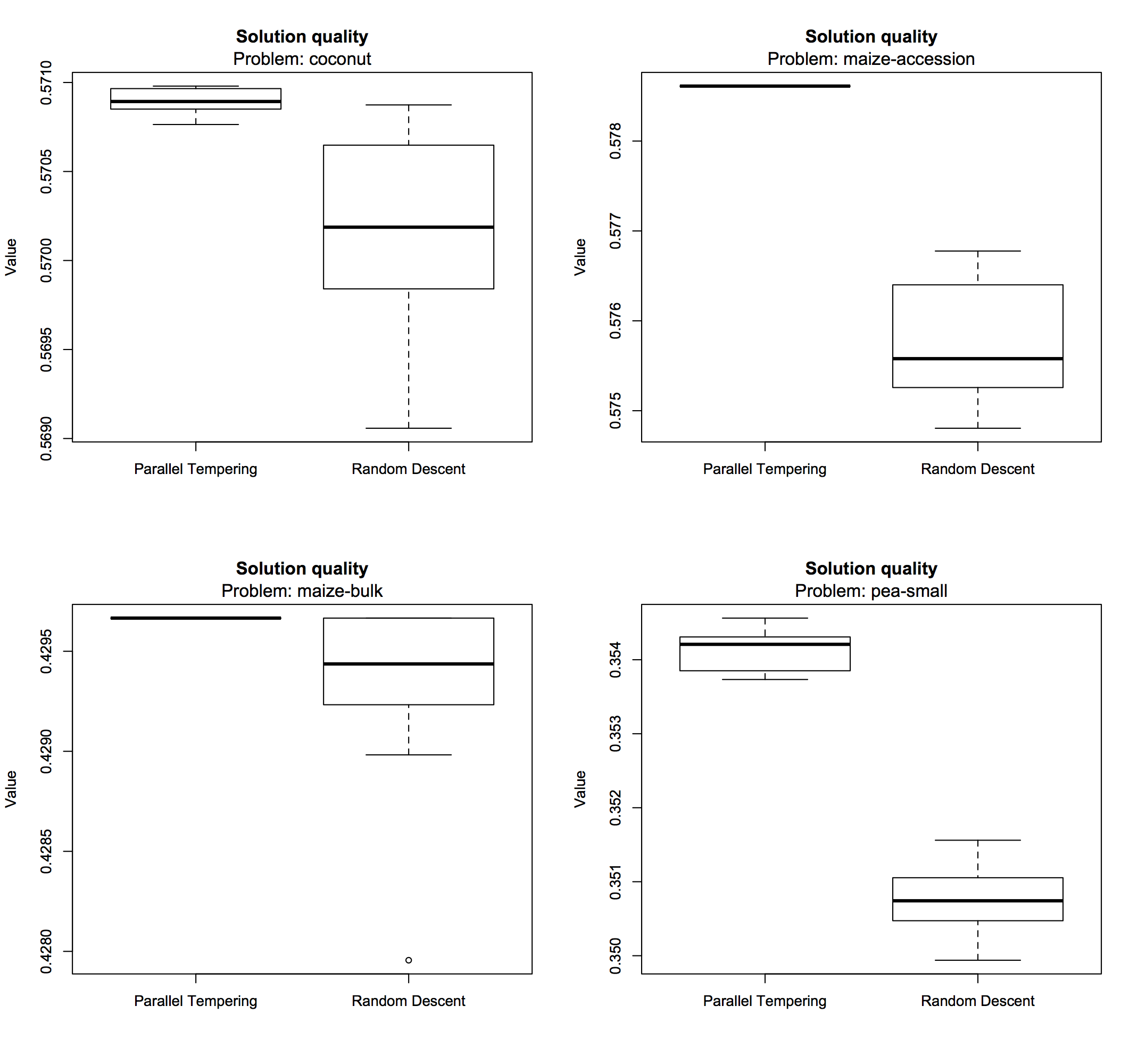
It is immediately clear that the parallel tempering algorithm produces slightly better results compared to random descent, with less variance across repeated search runs. Search performance can also be visualized using box plots:

> boxplot(comp, problem = "coconut")
> boxplot(comp, problem = "maize-accession")
> boxplot(comp, problem = "maize-bulk")
> boxplot(comp, problem = "pea-small")

Besides obtained solution quality, execution time is also an important characteristic of an optimization algorithm. The following box plots show how much time was spent until the search process converged, within the applied time limit of 15 minutes, across subsequent runs:

> boxplot(comp, problem = "coconut", type = "time", time.unit = "sec")
> boxplot(comp, problem = "maize-accession", type = "time", time.unit = "sec")
> boxplot(comp, problem = "maize-bulk", type = "time", time.unit = "sec")
> boxplot(comp, problem = "pea-small", type = "time", time.unit = "sec")

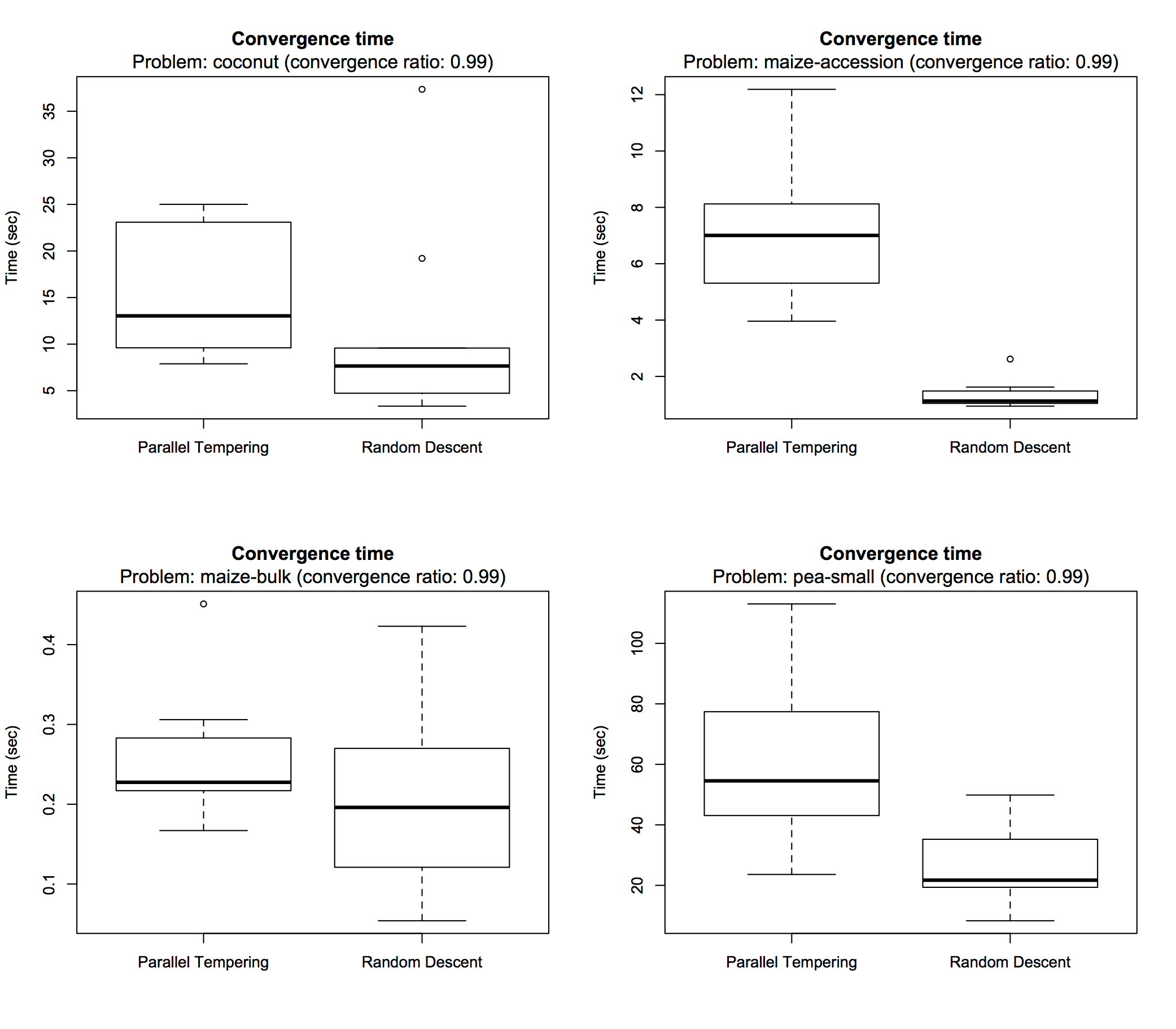
By default a convergence ratio of 0.99 is used for such visualizations, meaning that the point in time is reported at which 99% of the progress from initial to final solution has been made. Setting the convergence ratio to 1 reports the precise time at which the final best solution was found. In this experiment, all search runs converged within at most a few minutes (often seconds) with random descent being generally faster than parallel tempering (which is of course expected for an advanced algorithm).

The function plotConvergence provides a different way to visualize convergence. For example, for the pea collection it produces:

> plotConvergence(comp, problem = "pea-small", time.unit = "sec")

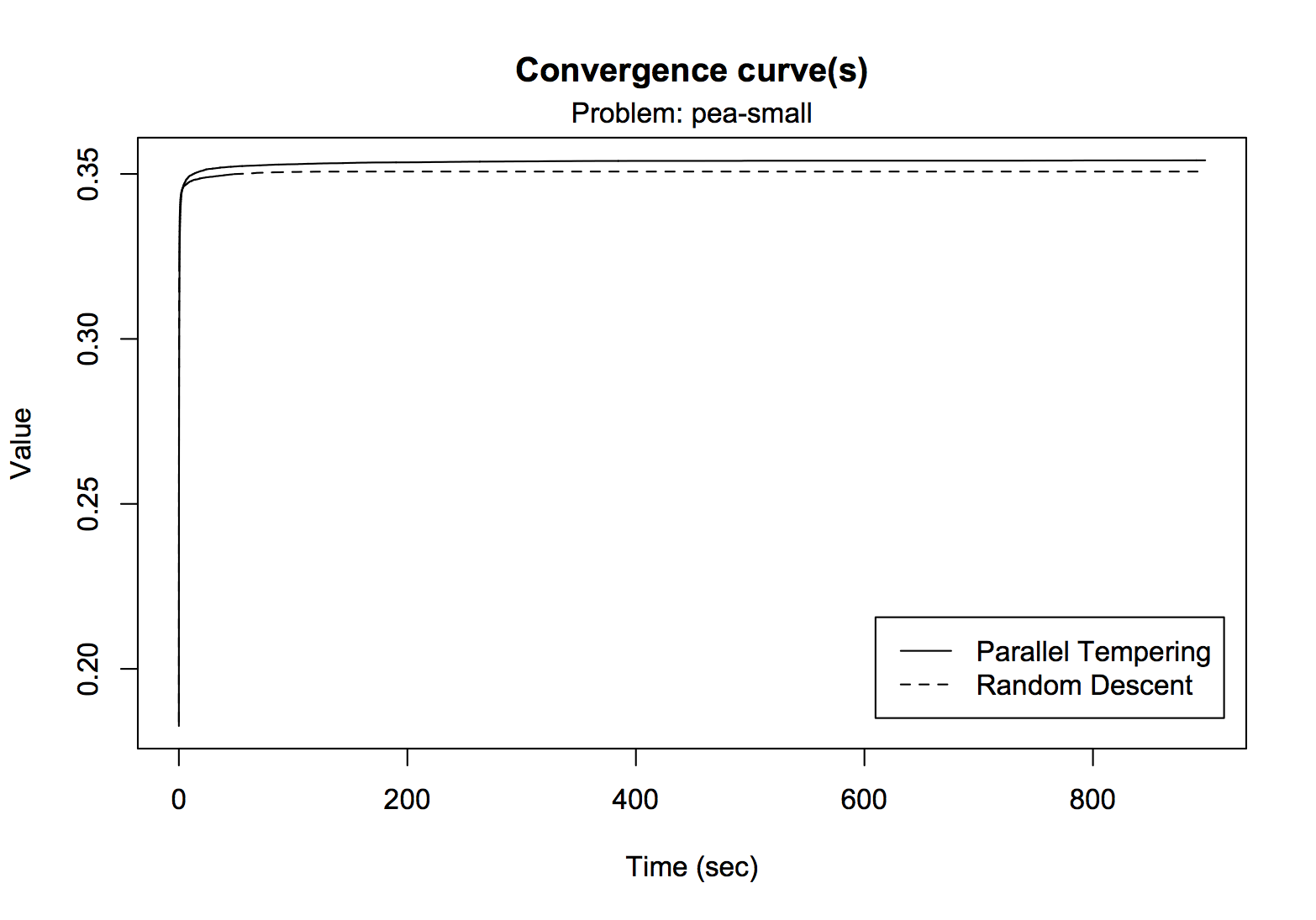
The graph again shows that parallel tempering reaches a slightly higher convergence plateau compared to random descent and that convergence occurs quite early for both algorithms. However, it is difficult to see what happens in the early stage of execution. The optional arguments min.time and max.time can be used to zoom in on a particular area of the curve, for example:

# combine 4 plots (2 x 2, by rows)
> par(mfrow = c(2,2))
# create plots with different zoom
> for(m in c(1,5,15)){
    plotConvergence(comp, problem = "pea-small", max.time = m, time.unit = "sec")
  }
> plotConvergence(comp, problem = "pea-small", min.time = 1, max.time = 10, time.unit = "sec")

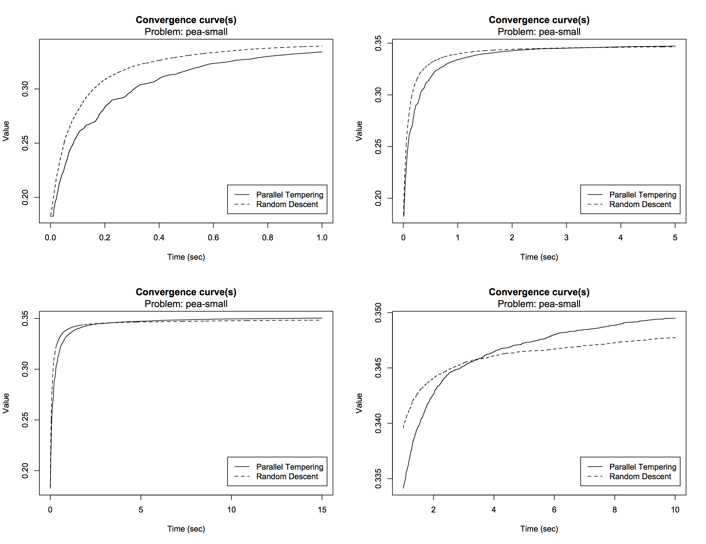
It is now clear that random descent takes a head start, improving the solution quality more rapidly than parallel tempering. After about 4 seconds, parallel tempering catches up and continues to improve the solution a little bit, reaching a slightly higher convergence plateau. If desired, data can easily be extracted from the results for further processing. Take a look at the following functions:

• getProblems
• getSearches
• getSearchRuns
• getBestSolutions
• getBestSolutionValues
• getConvergenceTimes

Documentation of all functions is available through ?<function>, e.g. try ?getBestSolutionValues. The R software is a very powerful tool for data analysis, even more so because of the vast amount of third-party packages. For example, we can easily perform some statistical tests to draw a more strongly supported conclusion.

# load library for exact Wilcoxon rank sum test
# if necessary install with 'install.packages("exactRankTests")'
> library(exactRankTests)

# extract final solution values obtained by random descent
> rd.values <- lapply(getProblems(comp), function(p){
    getBestSolutionValues(comp, problem = p, search = "Random Descent")
  })
# extract final solution values obtained by parallel tempering
> pt.values <- lapply(getProblems(comp), function(p){
    getBestSolutionValues(comp, problem = p, search = "Parallel Tempering")
  })
# compute p-value of Wilcoxon rank sum test (for each problem)
> p.values <- numeric(length(rd.values))
> for(i in 1:4){
    p.values[i] <- wilcox.exact(rd.values[[i]], pt.values[[i]])$p.value
  }
# adjust p-values for multiple testing (control FWER)
> p.adjust(p.values)

For each analyzed problem, the values of the best found solutions in subsequent runs of both algorithms are extracted. A Wilcoxon rank sum test is then applied to compare the results of the algorithms, which yields one p-value per dataset. The obtained p-values are adjusted for multiple testing to control the family-wise error rate (FWER) which gives the following values:

[1] 2.598021e-04 4.330035e-05 3.095975e-03 4.330035e-05

For each considered dataset, we can confidently reject the null hypothesis that the values obtained by random descent and parallel tempering were sampled from the same distribution, at the α = 0.05 confidence level. We conclude that parallel tempering tends to produce higher quality solutions than random descent for this problem. Yet, for the considered problem, the relative differences are small (always less than 1%, see results summary).

Full source code

The complete source code of this example is available on GitHub. You can also download a ZIP file that contains the Java sources of all examples, a compiled JAR (including all dependencies) as well as some input files for in case you want to run any of the examples. To run this example, execute

$ java -cp james-examples.jar org.jamesframework.examples.analysis.AlgoComparison <selectionratio> <runs> <runtime> [ <inputfile> ]+

from the command line. The selection ratio determines the core size. The following arguments specify the number of runs (repeats) that will be performed for each search and the runtime limit (in seconds) of each run. The input files (at least one) should be CSV files in which the first row contains N item names and the subsequent N rows specify an N × N distance matrix. The analysis will be repeated for each dataset loaded from the given files. All output is combined into a single file comparison.json that can be loaded in R using the provided R package.

Input files (ZIP)